Documents
 CV
CVWeierstrass-Durand-Kerner Iteration
General Remarks on GZIP Compression
High-Performance Computing with Xilinx Accelerator Cards
Machine Learning Cheatsheet; online: link
 CV
CVWeierstrass-Durand-Kerner Iteration
General Remarks on GZIP Compression
High-Performance Computing with Xilinx Accelerator Cards
Machine Learning Cheatsheet; online: link
All remaining zero points are denoted by \(\zeta_i\). A dynamically change of the \(\zeta_j\) in each iteration further accelerates the convergence. Therefore, dataraces can be ignored.
The iteration breaks after \(10d\) runs, or if for a user given \(\varepsilon > 0\) the equation
holds. This iteration is commonly known as Weierstraß-Durand-Kerner Iteration. The zero points are converted in coordinates in a \(1080 \times 1080\) pixel image. In the end, the image is generated on the CPU in ppm format. Figure 1 shows an example.


left: \(n=30\times 10^6\), \(d=8\), real part of coefficients \(\pm\)1; right: \(n=30\times 10^6\), \(d=8\), imaginary part of coefficients \(\pm\)1


left: \(n=60\times 10^6\), \(d=4\), real part of coefficients \(\pm\)1; right: \(n=40\times 10^6\), \(d=12\), imaginary part of coefficients \(\pm\)1
Figure 1: Graphical representation of zero points in complex plane (\(1080 \times 1080\) pixel, \(\varepsilon=0.0001\)). The zero points are approximately distributed on a circle with radius one.
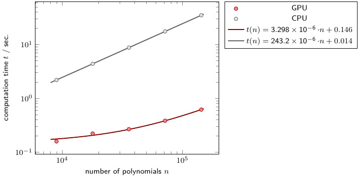
Figure 2: Computation times \(T\) for certain numbers of polynomials \(n\).
In the last step the dependency on the polynomial degree is evaluated (Fig. 3). When the degree is doubled, for the same number of polynomials twice the number of zero points are required in order to keep the overall number constant. The number of floating point operations and the iterations increase also with the degree. For degree 8 and 32 the computation time is almost the same for a larger number of polynomials.
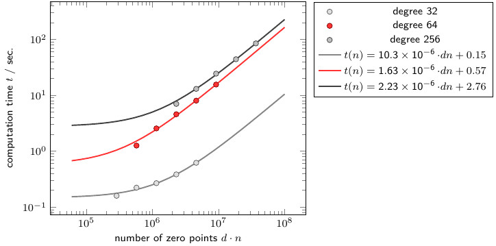
Figure 3: Computation times \(t\) for certain number of zero points \(dn\).
Source code at github.com.
Documentation
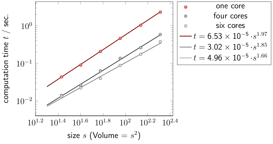
Figure 4: Comparison of computation times depending on the grid size \(s\) for different number of MPI processes.
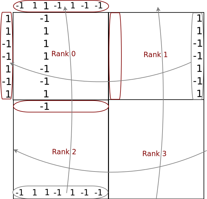
Figure 5: Visualization of the exchange of the boundary values (for 4 MPI processes).
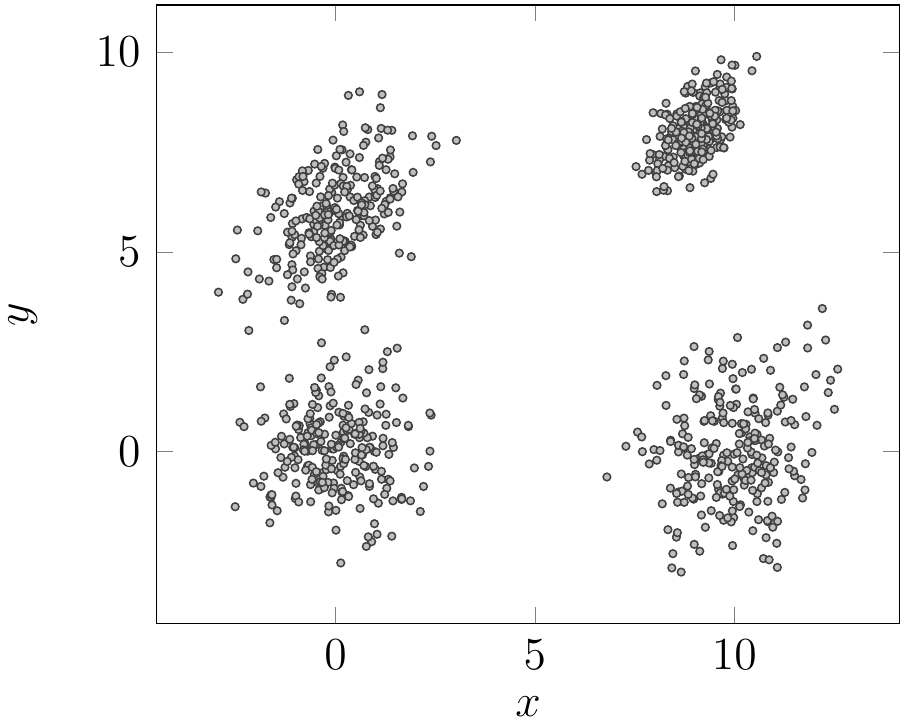
Figure 6: Four different clusters sampled randomly via gaussian mixture models. Each cluster consists of 250 two-dimensional points.
After tuning the parameters outliers can be detected and filtered:
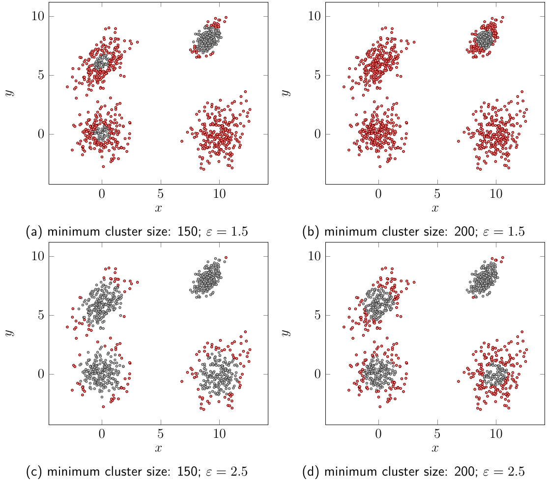
Figure 7: Outliers (red) and clusters (gray)
The main advantages of the algorithm are:
